Director: Joseph J. Luczkovich, PhD
Coastal Resources Management Program
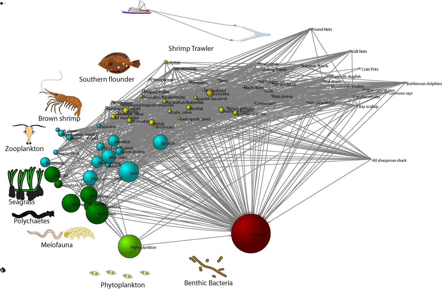
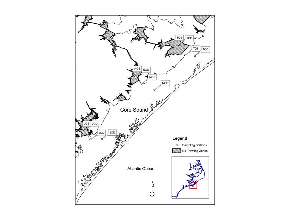
The impacts of commercial trawling are well documented, especially alteration of benthic environments, removal of targeted and by-catch species, and alteration of food webs. I investigated and modeled the impacts of shrimp trawling on the estuarine ecosystem in Core Sound, North Carolina. Since 1978, the North Carolina Division of Marine Fisheries has enforced no-trawling rules in nursery areas, but most of Core Sound is open to trawling. This “natural experiment” allowed me to compare the ecosystem impacts trawling using ecological network models. I used field collections, fisheries data from the NC Trip Ticket program, and Ecopath network modeling software to create four network models of areas open and closed to shrimp trawling during spring (2007) and fall (2006 and 2007). Each model consisted of 65 compartments (including non-living detritus, by-catch, producers, and various invertebrate and vertebrate consumers), and harvests by different types of fishery gears (crab pots, gill nets, haul seines, and pound nets in closed areas; shrimp trawls, skimmer trawls were added to the models in areas open to trawling).
Approximately 12,000 shrimp trawling trips occurred from 2001 – 2007 in areas open to trawling, suggesting the potential for large trawling impacts. Based on the benthic sampling, shrimp trawling had a major impact on the Core Sound ecosystem. Contrary to expectation, biomass (g C/m2) of infaunal benthic invertebrates, especially deposit-feeding polychaetes, was significantly greater in areas open to trawling. Meiofaunal biomass was significantly greater in the closed areas. Field collections of fish and invertebrates revealed that there was more biomass (g C/m2) of benthic-invertebrate feeders (such as spot, pinfish and blue crabs) in areas closed to trawling. These results suggest a trophic cascade due to trawling may have occurred in the open areas, whereby trawls removed benthic-feeding fishes and blue crabs, released their prey (benthic polychaetes) from predation pressure, and lowered the abundance of meiofauna (prey of the polychaetes). Alternatively, the dead biomass from by-catch could fuel the growth in polychaetes and other benthos due to a direct subsidy from trawling. Further experimental work is required to test these model-derived hypotheses.
Ecopath outputs were validated using stable isotopes and examined for system-wide impacts. The concentrations of stable isotopes of d15N and d13C were compared to Ecopath effective trophic levels. Trophic fractionation occurred across trophic levels, and results were comparable to published studies (for each unit effective trophic level increase there was a fractionation of +2.637‰ for d15N and +1.084‰ for d13C). Ecopath whole-ecosystem metrics indicated that net primary productivity, trophic efficiency, ascendency, and net primary production: respiration ratios were greater in the areas open to trawling; total system throughput and Finn Cycling Index were greater in the areas closed to trawling. Additional compartment-level comparisons were made using mixed trophic impacts (MTI) and keystoneness index (KSI). The MTI analysis indicated that shrimp trawling in Core Sound caused large negative impacts only on jellyfish, a bycatch species. The KSI indicated that sea turtles and brown pelicans were keystone groups (large influence relative to their biomass) overall in Core Sound. Spot, bluefish and Atlantic croaker also had high KSI in closed areas. Pink shrimp, white shrimp and bluefish all had high KSIs in the open areas, suggesting that they played a key role in the ecosystem’s trophic structure where trawling was allowed.
These Ecopath models can be useful tools for resource managers to better understand the direct and indirect impacts of (shrimp trawl) fishing in Core Sound. Future work should include the creation of annualized models and simulation modeling using Ecosim to explore different management scenarios.
Network model of Core Sound, NC, USA after the shrimping season in Fall 2007, model data from the areas open to trawling. The brown shrimp (Farfantepenaeus aztecus) fishery in North Carolina, valued at $13 million in 2012, depends on a food web comprised of detritus, bacteria, phytoplankton, seagrass, meiofauna, benthic polychaetes, and zooplankton. Shrimp are consumed by various fishes like the southern flounder (Paralichthys lethostigma). This graphic shows a multi-dimensional scaling statistical analysis of the feeding relationships observed in Core Sound, NC. The similarity of trophic roles of each species is shown by how close they plot together on the graph. Similarity was computed in terms of the regular role equivalence, the degree to which they consume or are consumed by species with similar trophic roles. Colors show species with similar feeding roles. The size of each node is proportional to the log 10-transformed biomass of the node in an Ecopath Network Model of the food web. Arrows show the flow of carbon from detritus to the top of the food web, represented here by the shrimp trawlers. This graphic uses a food web concept, which is a paragdigm commonly known to all students of ecology and scientists. The food web model was created using a computer modeling software (Ecopath) of the Core Sound estuarine system based on data from our own work, the literature, and the State of North Carolina. The visualization output was created with social network analysis software (UCInet), which was used to compute regular equivalence similarity coefficients and multi-dimensioanl scaling coordinates. The final network graph was made with Pajek. Organism and trawler images courtesy of Integration and Application Network, University of Maryland Center for Environmental Science (ian website at University of Maryland).
 |
 |
Sampling of Core Sound performed with benthic cores,
plankton net tows, otter trawls, barrier seines, wrap-around-net, and gill-nets.
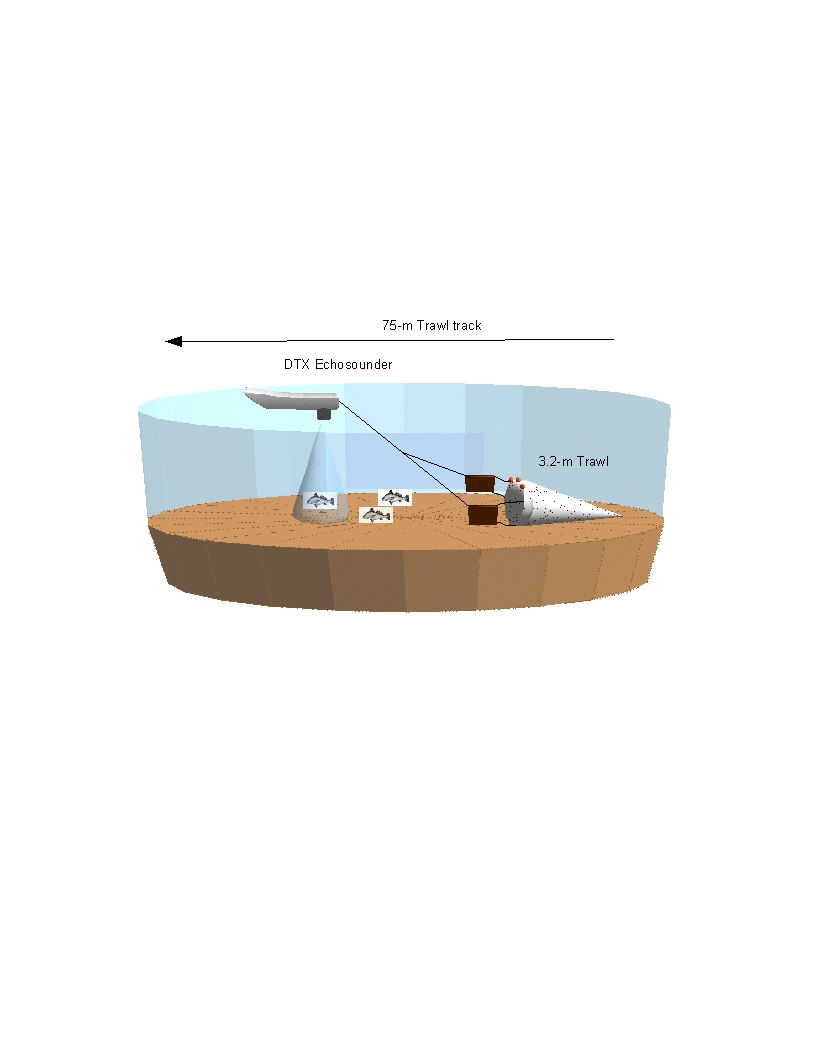
Trawling was performed using an otter trawl with a 3.2-m head-rope, 1-cm
stretched mesh in the wings and 3.2-mm stretch mesh cod end. Three two-minute
trawls covering approximately 75m were performed at each station.
Abundances (number of individuals/m2)
and biomass (g/m2) for each species were calculated after the samples
were measured and weighed. Trawl two
lengths were determined using a scientific echosounder operated simultaneously
with the trawl deployment. The
BioSonics DTX echosounder was used to assess bathymetry, bottom substrate, and
fish abundance in front of the trawl.
The echosounder was interfaced with a JVC GPS receiver and a Panasonic
Toughbook CF-29 laptop computer so that precise trawl tracks and depths were
recorded to a hard drive. Barrier
seining was performed in the methods similar to those performed by Christian and
Luczkovich (1999) and Luczkovich et al.
(2002). Barrier seines were used in
the fall 2006 and spring 2007. Biomass (g/m2) and number of
individual/m2 were calculated by assuming the area was constant
(A=1/2(b*h) =1/2(7.62*7.62) =29m2). The
gill nets were 114.3-m long with five 23-m panels of varying sizes. The panels
started at 8.9-cm and increased by 1.3-cm increments to 14-cm. Gill net sampling
area was determined assuming an area was sampled equal to the length of each
gill net squared (114.3m*114.3m =13,064.5 m2).
The strike net was 115-m long of # 10 monofilament twine
and 2.4m deep, with 8.9-cm stretch mesh, with the last 23 m were trammel net.
The strike net was deployed off the port side of the stern of the boat as the
boat was making a circle to enclose an area. Area
sampled after each wrap-around net was determined by using the routes from a
Garmin handheld 76S GPS and the Expert GPS software application.
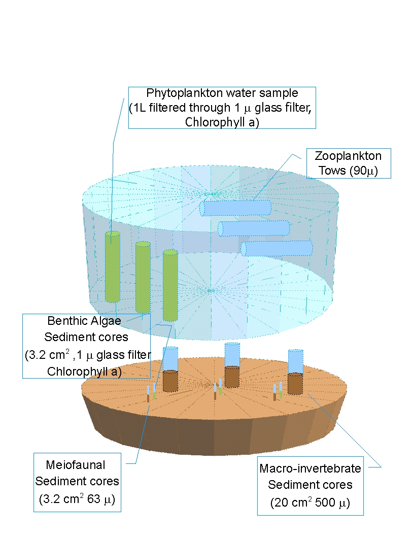
i. Benthic bacteria were collected using a 1-cm diameter syringe plunged to a depth of 1 cm and preserved in a scintillation vial filled with 19 ml of 2% bacteria-free formalin. Bacteria will be enumerated and biomass estimated by epiflourescence microscopy with 4’6-diamino-2-phenylinodole (DAPI) using a method similar to Marsh (2007), considering Schallenberg et al. (1989). All biomass measurements will be converted to grams Carbon using literature as necessary.
ii. Microalgae were collected using a 1-cm diameter syringe plunged to a depth of 1 cm, collected into a Whirlpak bag and stored on ice in a cooler until returned to the laboratory. Microalgae will be estimated from chlorophyll a content measured by fluorometry, similar to the methods of Baird et al. (1998). All biomass measurements will be converted to grams Carbon using literature as necessary.
iii. Sediment organic matter (for the detritus compartment) was collected using a 1-cm diameter syringe plunged to a depth of 1 cm, collected into a Whirlpak bag and stored on ice in a cooler until returned to the laboratory. Sediment organic matter will be measured by loss on ignition using the methods of Baird et al. (1998). All biomass measurements will be converted to grams Carbon using literature as necessary.
iv. Meiofauna were collected with a 2-cm diameter syringe plunged to a depth of 3 cm, and preserved in 10% buffered formalin with Rose Bengal. Meiofauna will be separated from sediments using the method of Burgess (2001), passed through a 63 μm sieve, and all specimens will be identified to lowest taxonomic level and measured for conversion to biomass (Higgins and Thiel 1988; Giere 1993). All biomass measurements will be converted to grams Carbon using literature as necessary.
v. Sediment samples were retained from the core (a “scoop” down to no more than 3 cm), collected into a Whirlpak bag and stored in a cooler until returned to the laboratory. The samples were dried in a 60°C oven for 48 hours, ground with a mortar and pestle to remove large clumps and processed in the Geology Department Ro-Tap machine for 10 minutes. Grain sizes were measured as the amount of a 100 g sample retained on sieves from 1.0 φ to 4.5 φ, corresponding to grain sizes of coarse sand to silt/clay, respectively.
To construct a diet matrix, diet data were collected using stomach content analysis for several fishes (Hart 2008), while diet information for all other compartments as gathered from literature. A sieve fractionation method (modified by Luczkovich and Stellwag [1993] from Carr and Adams [1973]) and used by Baird et al. (1998), Luczkovich et al. (2002) and Chagaris (2006) was used in this study.
Information on ecotrophic efficiency and production:biomass
and consumption:biomass ratios was collected from literature.
It was necessary to utilize existing datasets for this information
(Peters 1983; Jorgensen et al. 1991; Christensen and Pauly 1993; Christian and
Luczkovich 1999; Johnson 2006; Froese and Pauly 2006; Chagaris, unpublished
Ecopath model of Pamlico River estuary).
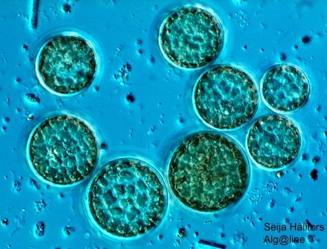 Diatoms
and algae Diatoms
and algae |
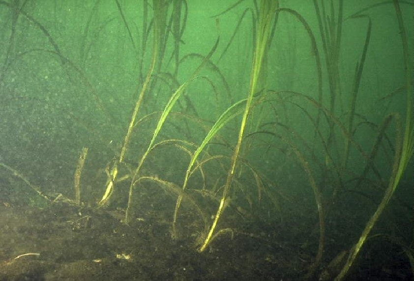 Seagrasses Seagrasses |
Producers |
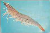 Penaeid
shrimp Penaeid
shrimp |
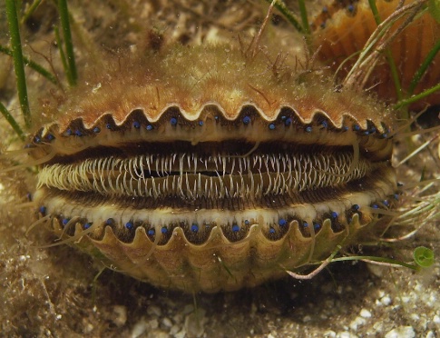 Bivalves
(scallops, clams, oysters) Bivalves
(scallops, clams, oysters) |
Herbivores |
|
|
|
Zooplanktivores |
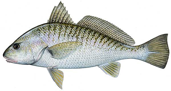 Atlantic
Croaker Atlantic
Croaker |
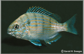 Pinfish Pinfish |
Benthic feeders |
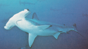 Sharks Sharks |
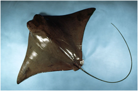 Rays Rays |
Apex predators |
Compartment Number and Name |
Species or pooled taxa |
|
1 |
Phytoplankton |
|
2 |
Microalgae_benthic |
|
3 |
Macroalgae_benthic |
Codium, Ruppia, Ulva |
4 |
Drift algae |
Gracilaria, Sargassum |
5 |
Seagrass |
Zostera, Halodule |
6 |
Bacteria_aquatic |
|
7 |
Bacteria_benthic |
|
8 |
Meiofauna |
harpacticoid copepods, foraminifera, nematodes, platyhelminths, tardigrades, ostracods, kinorhynchs, polychaetes, oligochaetes, amphipods |
9 |
Zooplankton |
Calanoid and cyclopoid copepods, holoplankton, meroplankton, other zooplankton |
10 |
Jellyfish |
|
11 |
Ctenophores |
|
12 |
Polychaetes_depfd |
Families: Capitellidae, Cirratulidae, Maldanidae, Opheliidae, Orbiniidae, Paraonidae, Pectinariidae, Terebellidae, Syllidae |
13 |
Polychaetes_suspfd |
Families: Poecilochaetidae, Sabellidae, Spionidae |
14 |
Polychaetes_pred |
Families: Amphinomidae, Eucinidae, Glyceridae, Goniadidae, Lumbrineridae, Phyllodocidae, Nereididae, Nemertea |
15 |
Bivalves_suspfd |
Genera Aesthenothaerus, Chione, Gemma, Lucina, Macoma, Nucula, Parvilucina, Tagelus, Tellina, Family Lasaeid |
16 |
Bay scallop |
Argopecten irradians |
17 |
Hard clam |
Mercenaria mercenaria |
18 |
Gastropods_depfd |
Astyris sp., Acteocina canaliculata |
19 |
Gastropods_pred |
Genera Eulimastoma, Polinices, Turbonilla, Family Nassarid |
20 |
Conchs/whelks |
|
21 |
Atl brief squid |
Lolliguncula brevis |
22 |
Bryozoans |
Bugula sp., Zoobotryon verticillatum |
23 |
Tunicates |
Styela sp. |
24 |
Sea cucumbers |
|
25 |
Brittlestars |
|
26 |
Amphipod/isopod/cumacean |
caprellid and gammarid amphipods, isopods and cumaceans |
27 |
Blue crabs |
Callinectes sapidus, C. similis |
28 |
Crabs_other |
small crabs in Brachyurid Superfamilies: Majoidea, Portunoidea, Xanthoidea, Pinnotheroidea, and Paguroidea |
29 |
Brown shrimp |
Farfantepenaeus aztecus |
30 |
Pink shrimp |
Farfantepenaeus duorarum |
31 |
White shrimp |
Litopenaeus setiferus |
32 |
Shrimps_other |
mantis, grass, and snapping shrimp |
33 |
Anchovies |
Anchoa mitchilli, A. hepsetus |
34 |
Atl croaker |
Micropogonias undulatus |
35 |
Atl menhaden |
Brevoortia tyrannus |
36 |
Atl silverside |
Menidia menidia |
37 |
Atl spadefish |
Chaetodipterus faber |
38 |
Black drum |
Pogonias chromis |
39 |
Bluefish |
Pomatomus saltatrix |
40 |
Flounders (Paralichthids) |
Paralichthys dentatus, P. lethostigma, P. albigutta |
41 |
Harvestfish/Butterfish |
Peprilus paru, P. triacanthus |
42 |
Striped mullet |
Mugil cephalus |
43 |
Pigfish |
Orthopristis chrysoptera |
44 |
Pinfish |
Lagodon rhomboides |
45 |
Pompano |
Trachinotus carolinus |
46 |
Red drum |
Sciaenops ocellatus |
47 |
Sheepshead |
Archosargus probatocephalus |
48 |
Southern kingfish |
Menticirrhus americanus |
49 |
Spanish mackerel |
Scomberomorus maculatus |
50 |
Spot |
Leiostomus xanthurus |
51 |
Spotted seatrout |
Cynoscion nebulosus |
52 |
Weakfish |
Cynoscion regalis |
53 |
Bottlenose dolphins |
Tursiops truncatus |
54 |
Sea turtles |
Caretta caretta |
55 |
Atl sharpnose shark |
Rhizoprionodon terraenovae |
56 |
Smooth dogfish |
Mustelus canis |
57 |
Cownose rays |
Rhinoptera bonasus |
58 |
Other rays/skates |
clearnose skate (Raja eglanteria), smooth butterfly ray (Gymnura micrura), bullnose ray (Myliobatis freminvillei), southern stingray (Dasyatis americana), spotted eagle ray (Aetobatus narinari) |
59 |
Brown pelicans |
Pelicanus occidentalis |
60 |
Cormorants |
Double-crested cormorant (Phalacrocorax auritus) |
61 |
Gulls |
black-backed (Larus marinus), herring (L. argentatus), and laughing gulls (Leucophaeus atricilla) |
62 |
Terns |
common (Sterna hirundo), royal (Thalasseus maximus), sandwich (T. sandvicensis) and least terns (Sternula antillarum) |
63 |
Shorebirds/waders |
great egret (Ardea alba), great blue heron (A. herodias), semipalmated plovers (Charadrius semipalmatus), semipalmated sandpipers (Calidris pusilla), black-bellied plovers (Pluvialis squatarola), green heron (Butorides virescens), tri-colored heron (Egretta tricolor), black skimmer (Rynchops niger) |
64 |
Bycatch |
See below |
65 |
Detritus |
|
Fishery Nodes, data sources and assumptions:
| ID | Node names | Data Sources, composition of catches and assumptions |
| 64 | Shrimp Trawl Bycatch |
From Johnson (2003), assume total bycatch is 5.7 to every 1 shrimp; spot 21%, croaker 8%, blue crabs 40%, pinfish 4%, silversides 2%, pigfish 2%, flounder 1%, harvestfish 1%, menhaden 1%, jellyfish 6%, other shrimps 6%, other crabs 6%, 2% anchovies |
| 64 | Skimmer Trawl Bycatch |
From Coale/Hines studies (1993, 1994), shrimp catch is 32% of total catch, so bycatch = spot (10.3%), croaker (0.9%), blue crabs (12.1%), pinfish (8.2%), silversides (0.2%), pigfish (1.7%), flounder (0.28%), harvestfish (0.08%), menhaden (6%), jellyfish (1.94%), other shrimps (1.94%), other crabs (1.94%), anchovies (1.1%), spadefish (0.4%), spotted seatrout (0.04%), weakfish (0.6%), stingrays (0.3%), squid (0.2%), smooth dogfish (0.8%), southern kingfish (0.04%), striped mullet (0.9%), bluefish (0.9%), Spanish mackerel (2.5%), pompano (0.1%), non-model others (10.66%) |
| 65 | Detritus | Dead decaying plant material |
| 66 | Imported Biomass | Assumed migration of larvae and fishes into Core Sound |
| 67 | Haul Seines |
maximum length (in regulations from VA.) of haul-seine, 1000 m; this forms circumference of circle with radius 159 m; area inside = 79,557 m2 (area fished) |
| 68 | Crab Pots |
200 pots/trip, 10 m radius/pot = 314.159 m2*200 = 62831.85 m2 (area fished) |
| 69 | Pound Nets |
average length of net lead, 500 m, radius of circle; area inside = 785,398 m2 (area fished) |
| 70 | All Gill Nets combined |
6000 yards/trip (two nets 3000 yards each) *100 yds each side = 1,200,000 sq yds or 1,003,352.832 m2 (area fished) |
| 71 | Shrimp Trawls |
90ft total headrope (27.432 m), six hauls (90 min tow plus 30 min cull during 12 hour period), travel speed of 2.25 mph for 90 min (5431.536 m distance) = 6*27.432 m*5431.536 m = 893,987 m2 (area fished) |
| 72 | Skimmer Trawls |
26 ft total headrope (7.925 m), towed continuously for 12 hours (no culling time), travel speed of 2.5 knots (or 4.63 km/hr) = 7.925 m*55.56 km*1000 m/km = 55,560 m2 (area fished) |